
My previous post walked through the code for implementing a general feedforward neural network program in Python. This post shows the program in action, applied to two classification problems. All of the code for this post is available here.
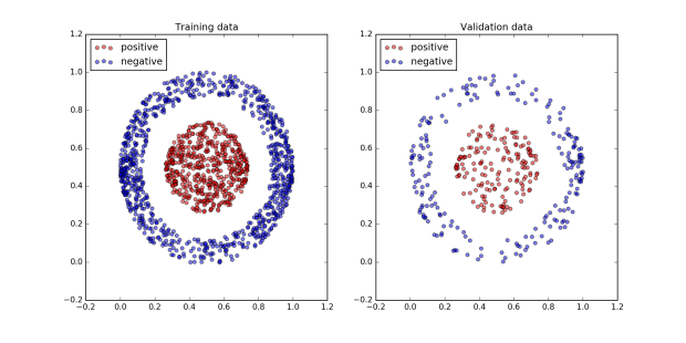
The first problem is to separate the red from the blue classes in the dataset pictured below. The code for generating and plotting the dataset is here. It’s a simple example but nicely demonstrates the power of neural networks.
Using the program is very simple. First the data needs to be loaded and the neural network initialized.
import pickle
%run NeuralNet2.ipynb

train_x = pickle.load( open( "nn_donutballdata_train_x.pkl", "rb" ) )
train_y = pickle.load( open( "nn_donutballdata_train_y.pkl", "rb" ) )
test_x = pickle.load( open( "nn_donutballdata_test_x.pkl", "rb" ) )
test_y = pickle.load( open( "nn_donutballdata_test_y.pkl", "rb" ) )

net = NeuralNet((2,4,1), QuadraticCost, SigmoidActivation,
                SigmoidActivation)
net.initialize_variables()
A brief aside about formatting data to use with this program. Any training or test data needs to be arranged as a 2D numpy matrix of floating point numbers of size m x n where m is the number of examples and n is the number of features (for input data) or labels (for output data). So in this example, in train_x and test_x, each column represents a feature and each row represents a single example. train_y and test_y are vectors in which each element represents the class of the corresponding example with a value of 1 for the positive class, 0 for the negative class. train_x is 1400 x 2 since there are two input features, the x and y coordinates of the data, and 1400 training examples. train_y is 1400 x 1 since there is one output label of interest. There are 372 examples reserved for the test set.
The last two lines are where all the work happens. First, a three layer neural network is initialized, with one input layer of 2 nodes, one for each input feature, one hidden layer of 4 nodes, and one output layer with 1 node, since we are interested in predicting the probability of a datapoint belonging to the positive class. The cost function the network is minimizing is the Quadratic Cost. The activation function in the hidden layer is the Sigmoid (2nd to last parameter, this sets the activation function for all hidden layers), as is the activation function in the output layer (last parameter). Then the last line initializes all of the network’s variables, the weights and the biases.
All that is needed now is to set the hyper-parameters and call the SGD function which trains the network through stochastic gradient descent.
learning_rate = 0.1
batch_size = 10
lmda = 0
epochs = 1001
reporting_rate = 200
training_cost, valid_cost = net.SGD(train_x, train_y,
                                    test_x, test_y,
                                    learning_rate,
                                    epochs,
                                    reporting_rate,
                                    lmda,
                                    batch_size)
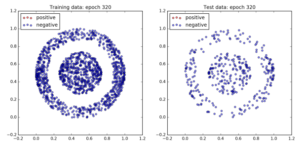
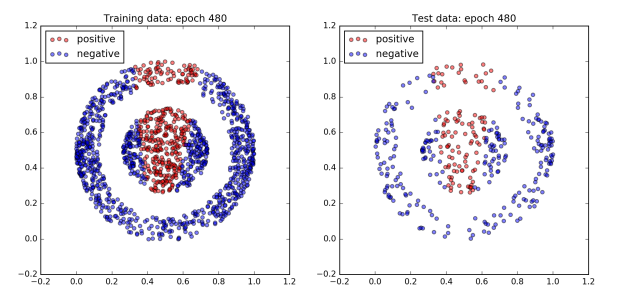
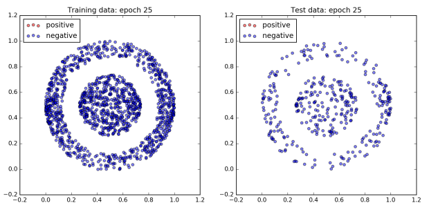
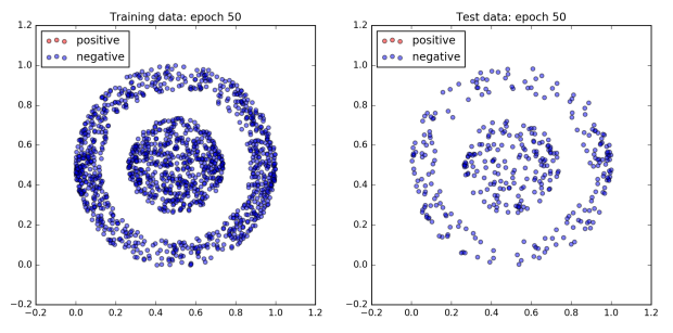
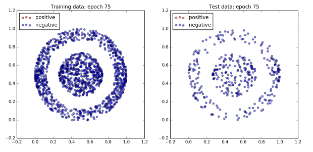
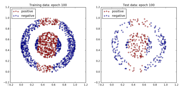
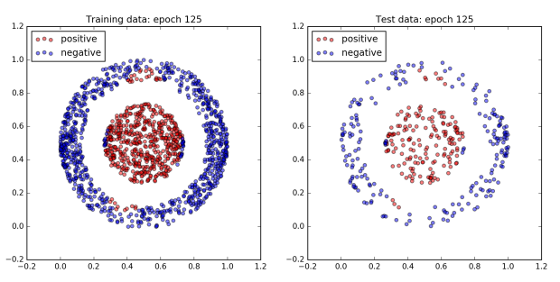
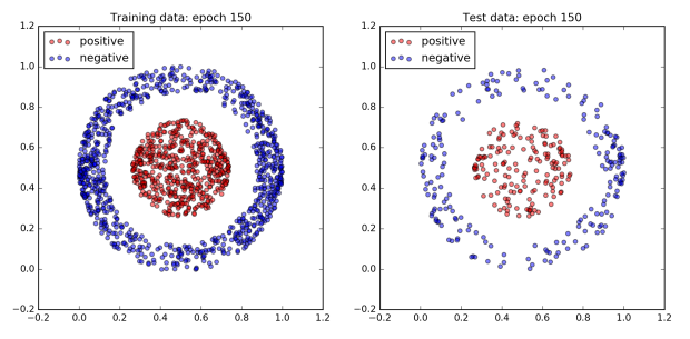
The figure below plots the network’s performance as training progresses. All of the dots in the inner ball should be colored red, and all of the dots in the outer ball should be colored blue.
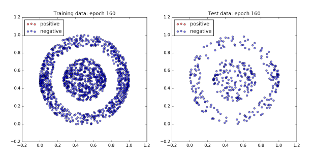
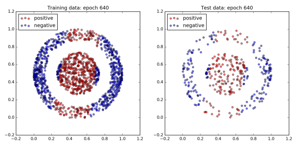
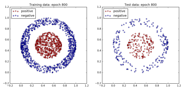
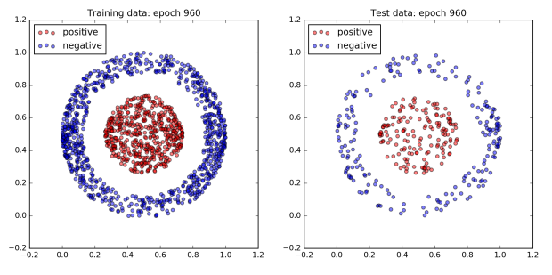
To begin with the network does not do very well and all of the dots are blue. However, after 960 epochs, the network achieves 100% accuracy on both the training and test dataset. Since a boundary exists which cleanly separates the two classes by design, this is to be expected.
Interestingly, not much happens for the first 300 epochs. Then by the 480th epoch the cost has dropped significantly and the accuracy has jumped up to approximately 80%. After that, accuracy sticks at around 80% for the next 300 or so epochs. However plotting the dataset reveals that quite a lot is changing behind the scenes. The images of epochs 480 and 640 show that during this time the decision boundary has shifted from a cone to a band. Finally, the accuracy jumps to 100% accuracy by the 800th epoch, and the decision boundary has converged on the correct one, a circle.
The lack of progress in the beginning is quite a common picture of training. Often learning is very slow for a while, then performance starts to improve, then it plateaus again, then it improves. Suggesting that the network is moving between flat regions of cost-parameter space where little progress is made and steep regions where large decreases in the cost function are possible. As a result, it can sometimes be difficult to work out if a network is in a flat region but will eventually start to learn, or if it will never learn anything at all.
One way to tackle this problem is to start with a small subset of the training data and a reasonably small network so that the network takes only 15 – 30 seconds per epoch to run. This makes it quick to iterate over different hyper-parameters until the network starts to learn something. Once you have established that the network can actually learn something it becomes much easier to make incremental improvements from that standpoint.
There are many possible hyper-parameter settings to play with and they have a significant effect on how fast a neural network learns. Or if it learns anything at all. Below is an example where the only differences when compared with the network above are the cost function and the methodology for initializing the network parameters. However it learns to separate this data about 80% faster, taking only 150 epochs to achieve 100% accuracy with the same learning rate and batch size.
net = NeuralNet((2,4,1), CrossEntropyCost, SigmoidActivation, SigmoidActivation)
net.initialize_variables_normalized()
learning_rate = 0.1
batch_size = 10
lmda = 0
epochs = 150
reporting_rate = 200
training_cost, valid_cost = net.SGD(train_x, train_y,
                                    test_x, test_y,
                                    learning_rate,
                                    epochs,
                                    reporting_rate,
                                    lmda,
                                    batch_size)
This jupyter notebook contains lots of examples which highlight the effect of different settings on network performance. They are by no means exhaustive but demonstrate how sensitive networks can be to different parameter initialization strategies, cost functions, batch sizes, and activation functions.
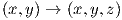
As well as adjusting the hyper-parameters, there is also the network architecture to consider. Since this is a very straightforward classification problem with a simple non linear boundary, I hypothesized that a neural network with just one hidden layer of a few nodes should be sufficient. However, the choice of four nodes was somewhat arbitrary. A more rigorous approach would be to consider the data transformation required for the classes to be linearly separable. A transformation which projected the x and y coordinates into three dimensions,
where z = 1 if,
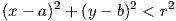
and z = 0 otherwise, would be sufficient. (a, b) is the center of the circle of red dots and r is the radius of a circle with origin (a,b), sufficient large to cleanly contain the red dots and exclude the blue dots. The result of this projection is to raise all of the points within the circle (red dots) above the blue dots when visualized in three dimensions. The plane specified by z = 0.5 would then separate the two classes. Reasoning about the data this way suggests that at least 3 nodes in the hidden layer are necessary, but would probably also be sufficient. This notebook shows that this is indeed the case.
Most of the time it is not so easy to reason about the architecture of a neural network. In practice finding the best architecture tends to be a result of trial and error. However, a general heuristic is that as problems become more complex, more layers are likely to be useful, since this makes it easier for the network to learn complex data transformations.
The second example is the classic MNIST dataset. This is a large set of grayscale 28 x 28 images of handwritten digits from 0-9, each with an associated label. The objective is to correctly classify each digit.
import pickle
%run NeuralNet2.ipynb
train_x = pickle.load(open("MNIST_train_x.pkl", 'rb'))
train_y = pickle.load(open("MNIST_train_y.pkl", 'rb'))
test_x = pickle.load(open("MNIST_test_x.pkl", 'rb'))
test_y = pickle.load(open("MNIST_test_y.pkl", 'rb'))
short_train_x = train_x[0:5000,:]
short_train_y = train_y[0:5000,:]

net2 = NeuralNet((784,100,10), LogLikelihoodCost, ReluActivation, SoftmaxActivation)
net2.initialize_variables()
learning_rate = 0.001
epochs = 61
reporting_rate = 20
lmda = 0
batch_size = 200
training_cost, valid_cost = net2.SGD(short_train_x, short_train_y,
                                     test_x, test_y,
                                     learning_rate,
                                     epochs,
                                     reporting_rate,
                                     lmda,
                                     batch_size,
                                     verbose=False)
The data is loaded as 2D numpy arrays, examples x features. Note that the images have been flattened from a 28 x 28 matrix into a vector in 784 dimensions, so that a single row can represent one image, and each column corresponds to one pixel. Even a small network like this takes a long time to train on a laptop with the full dataset. So to speed up training for a variety of different networks, I have selected the first 5,000 examples from the training data. Despite its simplicity, training a neural network with one hidden layer of 100 nodes with just 5,000 examples gives surprising good results, 90% accuracy on the test data.
The network is initialized with three layers; 784 input nodes, one for each pixel in the image, 100 hidden nodes, and 10 output nodes, one for each class. The ReLU activation function is used in the hidden layer, and softmax in the output layer. A softmax output layer has the benefit of outputting a probability distribution over each of the output classes. So the value of any output node for a particular example can be interpreted as the probability that the example belongs to the corresponding class. Softmax is best used with the log likelihood cost function, since it “undoes” the exponential in the softmax function.
After just 61 epochs, with a relatively large batch size, this network achieves 99.5% accuracy on the training data, and 90.54% on the test data. Note that this particular network is overfitting the training data, as the performance on the test data is 9% lower than on the training data. This is to be expected given that the training data only contains 5,000 examples and there is no regularization (lmda = 0). See here, here, and here for some notebooks which experiment with different cost, activation functions, batch sizes, learning rates and initialization strategies. There is a huge variety in performance.
It is interesting to experiment with different number and sizes of layers. Deep learning theory tells us that it should be possible to approximate a function with the same accuracy using fewer nodes and more layers. The results from these experiments support this. What was most interesting to me is that, ceteris paribus, varying the size and number of layers didn’t have a dramatic effect on performance. Almost all of the different networks achieved accuracy on the test set to within 1% of each other. I suspect this is because the training data set was so small, and was the limiting factor. I leave it to the reader to experiment with these networks using more data. The exception was the 5 layer neural network with 40 fewer nodes compared to the baseline. This network may benefit from training for more epochs.
My best result using three layers and only 20,000 training examples, was with this network.
short_train_x = train_x[0:20000,:]
short_train_y = train_y[0:20000,:]

net2 = NeuralNet((784,100,10), LogLikelihoodCost, ReluActivation,
                  SoftmaxActivation)
net2.initialize_variables_alt()
learning_rate = 0.0001
epochs = 101
reporting_rate = 20
lmda = 0.5
batch_size = 100
training_cost, valid_cost = net2.SGD(train_x, train_y,
                                     test_x, test_y,
                                     learning_rate,
                                     epochs,
                                     reporting_rate,
                                     lmda,
                                     batch_size,
                                     verbose=False)
It reached 96.19% accuracy on the test data after 101 epochs. Regularization also shrank the difference in performance between the training and test set to just 1.43%. Not bad.
I hope that you’ve enjoyed this post and found it useful. If you have any feedback please send me an email at contact [at] learningmachinelearning [dot] org.
