OpenAI Lab released

I’m really excited about the first major release of the OpenAI Lab. It’s an experimentation framework for reinforcement learning using the OpenAI Gym, Tensorflow, and Keras. We are currently porting it to pyTorch.

OpenAI Lab is created to do reinforcement learning (RL) like science – theorize, experiment. It provides an easy interface to the OpenAI Gym and deep learning libraries, with an automated experimentation and evaluation framework, and a number of customizable algorithms available out of the box.

For more information check out the docs and the code.

lab_demo_dqn

Getting started with Reinforcement Learning

Reinforcement learning is a fascinating family of algorithms that closely match our intuitions about the way humans learn. Perhaps the two most famous examples come from DeepMind. In December 2013, they announced a deep reinforcement learning algorithm that surpassed human expert performance on a number of Atari games. Then in March 2016, another algorithm, AlphaGo, defeated Lee Sedol, the world’s best player at Go, a game orders of magnitude more complex than chess. More recently, reinforcement learning has made its way into Dota, a fiendishly fast-paced multiplayer battlefield game.

In reinforcement learning, algorithms are agents, which act in environments. Actions change the environment and generate rewards (or punishments) for the agent which reinforce good behavior and discourage bad behavior. Agents learn through trial and error, and eventually figure out what good and bad actions are in different settings.

Working with these algorithms is fun because you get to reason about a broad range of issues that have natural counterpoints in human learning. For example,

  • How should the world (environment) be described? What information does an agent need to learn the problem we are asking it to solve? How granular should this information be, i.e. on what level does the agent perceive events?
  • How should your algorithm remember its experiences? Should it forget things? If so, how?
  • How should your algorithm balance repeating things it knows are good v.s. trying out new things in order to learn more?
  • How complex is the problem? So how much capacity (think compute power or flexibility) does your algorithm need? And can too much complexity inhibit learning?

Many of the classic reinforcement learning problems are simulations with a visual component or computer games. For example, below are a few snapshots of an agent at different stages of the learning process in the Lunar Lander environment from the OpenAI gym. This is another reason why reinforcement learning is interesting. You get to watch your algorithm learn in real time. Sometimes this can be painful, but often it is delightful and surprising. It offers insights into an algorithmic learning process that are not readily available for other problems.


If this introduction has piqued your interest, then here are a few links to get you started.

Theory

Practice

Work out at the OpenAI Lab: This is an experimentation framework for deep Reinforcement Learning (RL) using the OpenAI Gym, Tensorflow, and Keras. OpenAI Lab is created to do RL like science – theorize, experiment, so has an automated experimentation and evaluation framework. It is also intended to reduce the time it takes to get started learning RL, and implement algorithms. To do this it provides a modular set of components that correspond to the main RL concepts, as well as a number of customizable algorithms, available out of the box.

For supported environments, loading them takes one line of code, allowing users to focus on designing agents to operate in them. Currently supported environments are a selection those provided by the OpenAI gym

Deep neural networks for RL algorithms are equally easy to implement, through the agent classes. The following algorithms are available;

  • SARSA
  • DQN
  • Double DQN
  • Actor Critic
  • Deep Deterministic Policy Gradients

All users need to specify is the architecture (number and size of hidden layers) and a few hyper-parameters. Alternatively, if you want finer grained control over the network architecture, inheriting from the relevant class will mean that the training is handled for you.

rl/spec/*_experiment_specs.json controls the parameter settings for an experiment. Either tweak existing parameter settings, or design your own agent. Below is an example set of specs for the LunarLander environment with a deep Q-network.

A Neural Network Program in Python: Part II

My previous post walked through the code for implementing a general feedforward neural network program in Python. This post shows the program in action, applied to two classification problems. All of the code for this post is available here.

The first problem is to separate the red from the blue classes in the dataset pictured below. The code for generating and plotting the dataset is here. It’s a simple example but nicely demonstrates the power of neural networks.

DonutBallDataset

Using the program is very simple. First the data needs to be loaded and the neural network initialized.


import pickle
%run NeuralNet2.ipynb

train_x = pickle.load( open( "nn_donutballdata_train_x.pkl", "rb" ) )
train_y = pickle.load( open( "nn_donutballdata_train_y.pkl", "rb" ) )
test_x = pickle.load( open( "nn_donutballdata_test_x.pkl", "rb" ) )
test_y = pickle.load( open( "nn_donutballdata_test_y.pkl", "rb" ) )

net = NeuralNet((2,4,1), QuadraticCost, SigmoidActivation, 
                SigmoidActivation)
net.initialize_variables()

A brief aside about formatting data to use with this program. Any training or test data needs to be arranged as a 2D numpy matrix of floating point numbers of size m x n where m is the number of examples and n is the number of features (for input data) or labels (for output data). So in this example, in train_x and test_x, each column represents a feature and each row represents a single example. train_y and test_y are vectors in which each element represents the class of the corresponding example with a value of 1 for the positive class, 0 for the negative class. train_x is 1400 x 2 since there are two input features, the x and y coordinates of the data, and 1400 training examples. train_y is 1400 x 1 since there is one output label of interest. There are 372 examples reserved for the test set.

The last two lines are where all the work happens. First, a three layer neural network is initialized, with one input layer of 2 nodes, one for each input feature, one hidden layer of 4 nodes, and one output layer with 1 node, since we are interested in predicting the probability of a datapoint belonging to the positive class. The cost function the network is minimizing is the Quadratic Cost. The activation function in the hidden layer is the Sigmoid (2nd to last parameter, this sets the activation function for all hidden layers), as is the activation function in the output layer (last parameter). Then the last line initializes all of the network’s variables, the weights and the biases.

All that is needed now is to set the hyper-parameters and call the SGD function which trains the network through stochastic gradient descent.


learning_rate = 0.1
batch_size = 10
lmda = 0
epochs = 1001
reporting_rate = 200
training_cost, valid_cost = net.SGD(train_x, train_y, 
                                    test_x, test_y,
                                    learning_rate, 
                                    epochs, 
                                    reporting_rate, 
                                    lmda, 
                                    batch_size)

The figure below plots the network’s performance as training progresses. All of the dots in the inner ball should be colored red, and all of the dots in the outer ball should be colored blue.

DonutBall_slowlearning-0

DonutBall_slowlearning-1

DonutBall_slowlearning-2

DonutBall_slowlearning-3

DonutBall_slowlearning-4

DonutBall_slowlearning-5

To begin with the network does not do very well and all of the dots are blue. However, after 960 epochs, the network achieves 100% accuracy on both the training and test dataset. Since a boundary exists which cleanly separates the two classes by design, this is to be expected.

Interestingly, not much happens for the first 300 epochs. Then by the 480th epoch the cost has dropped significantly and the accuracy has jumped up to approximately 80%. After that, accuracy sticks at around 80% for the next 300 or so epochs. However plotting the dataset reveals that quite a lot is changing behind the scenes. The images of epochs 480 and 640 show that during this time the decision boundary has shifted from a cone to a band. Finally, the accuracy jumps to 100% accuracy by the 800th epoch, and the decision boundary has converged on the correct one, a circle.

The lack of progress in the beginning is quite a common picture of training. Often learning is very slow for a while, then performance starts to improve, then it plateaus again, then it improves. Suggesting that the network is moving between flat regions of cost-parameter space where little progress is made and steep regions where large decreases in the cost function are possible. As a result, it can sometimes be difficult to work out if a network is in a flat region but will eventually start to learn, or if it will never learn anything at all.

One way to tackle this problem is to start with a small subset of the training data and a reasonably small network so that the network takes only 15 – 30 seconds per epoch to run. This makes it quick to iterate over different hyper-parameters until the network starts to learn something. Once you have established that the network can actually learn something it becomes much easier to make incremental improvements from that standpoint.

There are many possible hyper-parameter settings to play with and they have a significant effect on how fast a neural network learns. Or if it learns anything at all. Below is an example where the only differences when compared with the network above are the cost function and the methodology for initializing the network parameters. However it learns to separate this data about 80% faster, taking only 150 epochs to achieve 100% accuracy with the same learning rate and batch size.


net = NeuralNet((2,4,1), CrossEntropyCost, SigmoidActivation, SigmoidActivation)
net.initialize_variables_normalized()
learning_rate = 0.1
batch_size = 10
lmda = 0
epochs = 150
reporting_rate = 200
training_cost, valid_cost = net.SGD(train_x, train_y, 
                                    test_x, test_y, 
                                    learning_rate, 
                                    epochs, 
                                    reporting_rate, 
                                    lmda, 
                                    batch_size)

DonutBall_fastlearning-0

DonutBall_fastlearning-1

DonutBall_fastlearning-2

DonutBall_fastlearning-3

DonutBall_fastlearning-4

DonutBall_fastlearning-5

This jupyter notebook contains lots of examples which highlight the effect of different settings on network performance. They are by no means exhaustive but demonstrate how sensitive networks can be to different parameter initialization strategies, cost functions, batch sizes, and activation functions.

As well as adjusting the hyper-parameters, there is also the network architecture to consider. Since this is a very straightforward classification problem with a simple non linear boundary, I hypothesized that a neural network with just one hidden layer of a few nodes should be sufficient. However, the choice of four nodes was somewhat arbitrary. A more rigorous approach would be to consider the data transformation required for the classes to be linearly separable. A transformation which projected the x and y coordinates into three dimensions,

MathsEq0x

where z = 1 if,

MathsEq1x

and z = 0 otherwise, would be sufficient. (a, b) is the center of the circle of red dots and r is the radius of a circle with origin (a,b), sufficient large to cleanly contain the red dots and exclude the blue dots. The result of this projection is to raise all of the points within the circle (red dots) above the blue dots when visualized in three dimensions. The plane specified by z = 0.5 would then separate the two classes. Reasoning about the data this way suggests that at least 3 nodes in the hidden layer are necessary, but would probably also be sufficient. This notebook shows that this is indeed the case.

Most of the time it is not so easy to reason about the architecture of a neural network. In practice finding the best architecture tends to be a result of trial and error. However, a general heuristic is that as problems become more complex, more layers are likely to be useful, since this makes it easier for the network to learn complex data transformations.

The second example is the classic MNIST dataset. This is a large set of grayscale 28 x 28 images of handwritten digits from 0-9, each with an associated label. The objective is to correctly classify each digit.


import pickle
%run NeuralNet2.ipynb
train_x = pickle.load(open("MNIST_train_x.pkl", 'rb'))
train_y = pickle.load(open("MNIST_train_y.pkl", 'rb'))
test_x = pickle.load(open("MNIST_test_x.pkl", 'rb'))
test_y = pickle.load(open("MNIST_test_y.pkl", 'rb'))
short_train_x = train_x[0:5000,:]
short_train_y = train_y[0:5000,:]

net2 = NeuralNet((784,100,10), LogLikelihoodCost, ReluActivation, SoftmaxActivation)
net2.initialize_variables()
learning_rate = 0.001
epochs = 61
reporting_rate = 20
lmda = 0
batch_size = 200
training_cost, valid_cost = net2.SGD(short_train_x, short_train_y, 
                                     test_x, test_y, 
                                     learning_rate,
                                     epochs, 
                                     reporting_rate, 
                                     lmda, 
                                     batch_size, 
                                     verbose=False)

The data is loaded as 2D numpy arrays, examples x features. Note that the images have been flattened from a 28 x 28 matrix into a vector in 784 dimensions, so that a single row can represent one image, and each column corresponds to one pixel. Even a small network like this takes a long time to train on a laptop with the full dataset. So to speed up training for a variety of different networks, I have selected the first 5,000 examples from the training data. Despite its simplicity, training a neural network with one hidden layer of 100 nodes with just 5,000 examples gives surprising good results, 90% accuracy on the test data.

The network is initialized with three layers; 784 input nodes, one for each pixel in the image, 100 hidden nodes, and 10 output nodes, one for each class. The ReLU activation function is used in the hidden layer, and softmax in the output layer. A softmax output layer has the benefit of outputting a probability distribution over each of the output classes. So the value of any output node for a particular example can be interpreted as the probability that the example belongs to the corresponding class. Softmax is best used with the log likelihood cost function, since it “undoes” the exponential in the softmax function.

After just 61 epochs, with a relatively large batch size, this network achieves 99.5% accuracy on the training data, and 90.54% on the test data. Note that this particular network is overfitting the training data, as the performance on the test data is 9% lower than on the training data. This is to be expected given that the training data only contains 5,000 examples and there is no regularization (lmda = 0). See here, here, and here for some notebooks which experiment with different cost, activation functions, batch sizes, learning rates and initialization strategies. There is a huge variety in performance.

It is interesting to experiment with different number and sizes of layers. Deep learning theory tells us that it should be possible to approximate a function with the same accuracy using fewer nodes and more layers. The results from these experiments support this. What was most interesting to me is that, ceteris paribus, varying the size and number of layers didn’t have a dramatic effect on performance. Almost all of the different networks achieved accuracy on the test set to within 1% of each other. I suspect this is because the training data set was so small, and was the limiting factor. I leave it to the reader to experiment with these networks using more data. The exception was the 5 layer neural network with 40 fewer nodes compared to the baseline. This network may benefit from training for more epochs.

My best result using three layers and only 20,000 training examples, was with this network.


short_train_x = train_x[0:20000,:]
short_train_y = train_y[0:20000,:]

net2 = NeuralNet((784,100,10), LogLikelihoodCost, ReluActivation, 
                  SoftmaxActivation)
net2.initialize_variables_alt()
learning_rate = 0.0001
epochs = 101
reporting_rate = 20
lmda = 0.5
batch_size = 100
training_cost, valid_cost = net2.SGD(train_x, train_y, 
                                     test_x, test_y, 
                                     learning_rate,
                                     epochs, 
                                     reporting_rate, 
                                     lmda, 
                                     batch_size, 
                                     verbose=False)

It reached 96.19% accuracy on the test data after 101 epochs. Regularization also shrank the difference in performance between the training and test set to just 1.43%. Not bad.

I hope that you’ve enjoyed this post and found it useful. If you have any feedback please send me an email at contact [at] learningmachinelearning [dot] org.

A Neural Network program in Python: Part I

Following on from an Introduction to Neural Networks and Regularization for Neural Networks, this post provides an implementation of a general feedforward neural network program in Python. Writing the code taught me a lot about neural networks and it was inspired by Michael Nielsen’s fantastic book Neural Networks and Deep Learning.

Whilst reasonably short, and containing no error checking, the program is quite powerful. The network can be of an arbitrary size and it is a vectorized implementation, which significantly speeds up the network computation. That is, batches of data are processed through the network in one pass. The input data is a 2D matrix, in which each row corresponds to an example and each column corresponds to a feature. The output is also a 2D matrix, in which each row corresponds to an example and each column corresponds to an output.

Four activation functions are available: the Sigmoid, ReLU, LeakyReLU and Softmax. It is possible to specify a different activation function for the hidden and output layers. Three cost functions are available: Quadratic, Cross Entropy, and Log Likelihood, and three different parameter initializers. The network is trained using Stochastic Gradient Descent and a user has the freedom to specify the learning rate, batch size and degree of L2 regularization through the lmda parameter. This program also shows how modular neural networks are, and makes it easy to add additional activation, cost, or parameter initialization functions.

The most important parts of the program are included below with an explanation of the main steps. It assumes an intermediate understanding of Python and Object-Oriented Programming. The full code is available here.

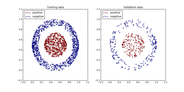
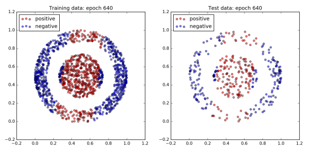
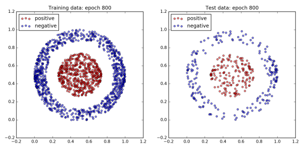
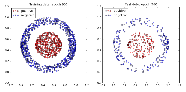
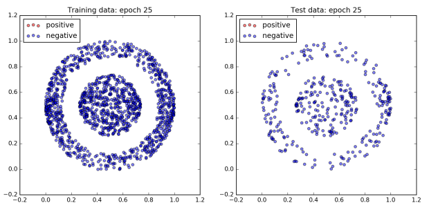
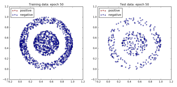
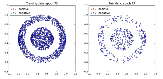
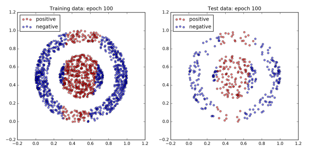
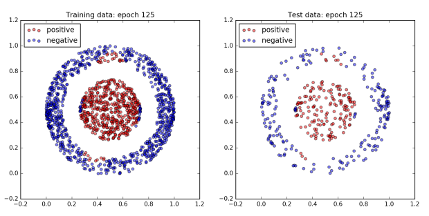
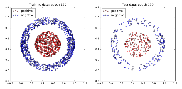
Part 2 of this post will give some examples of this program applied to solve two typical prediction problems. The first is a very simple three layer neural network used to solve a two class classification problem. The second are some example network structures and hyper-parameter settings applied to the classic MNIST computer vision task.

If you really want to understand neural networks, I highly recommend building your own. This program is intended as a reference to help readers do so, and to provide guidance when stuck. My next post will include tips for writing your own program as well as some suggested tests, and associated code, to run as you go.

Setup: Building the architecture of the neural network and initializing the variables


class NeuralNet:
    def __init__(self, size, costfn=QuadraticCost,
                 activationfnHidden=SigmoidActivation,
                 activationfnLast=SigmoidActivation):
        self.weights = []
        for a, b in zip(size[:-1], size[1:]):
            self.weights.append(np.zeros((a,b)))
        self.biases = []
        for b in size[1:]:
            self.biases.append(np.zeros((1, b)))
        self.layers = len(size)
        self.costfn = costfn
        self.activationfnHidden = activationfnHidden
        self.activationfnLast = activationfnLast
        
    def initialize_variables(self):
        np.random.seed(1)
        i = 0
        for w in self.weights:
            self.weights[i] = Matrix((np.random.uniform(-1, 1, 
                         size=w.shape) / np.sqrt(w.shape[0])))
            i += 1
        i = 0
        for b in self.biases:
            self.biases[i] = Matrix(np.random.uniform(-1, 1, 
                                    size=b.shape))
            i += 1

class Matrix:
    def __init__(self, matrix):
        self.matrix = matrix
    
    def __mul__(self, other):
        return Matrix(np.dot(self.matrix, other.matrix))
    
    def __add__(self, other):
        return Matrix(self.matrix + other.matrix)
    
    def __radd__(self, other):
        return Matrix(self.matrix + other.matrix)

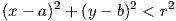
The first task is to build the network structure. size is a list containing the size of each layer, in order. So, size=(10, 5, 2) is a three layer neural network with one input layer containing 10 nodes, one hidden layer containing 5 nodes and one output layer containing 2 nodes. This information is used to create the weight matrices and bias vectors. The size of the n-th weight matrix is m x r, where m is the number of edges in the n-1 layer and r is the number of edges in the n-th layer. The number of weight matrices is therefore one fewer than the number of layers. Input nodes do not have biases. Bias vectors for the remaining layers have the same number of elements as nodes in a layer.

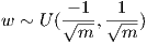
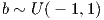
The rest of the initialization is straightforward. The attributes of the instance of the Neural Net class are set to the specified cost function, hidden layer(s) activation function (activationfnHidden) and output layer activation function (activationfnLast). The default settings are the quadratic cost function and sigmoid activation function for the hidden and output layers. Finally initialize_variables(self) initializes the weights and biases drawn from a uniform distribution centered around 0. Let w be any weight in the network, and b be any bias, and let m be the number of inputs to nodes in the layer that w is associated with. Then we have,

NNProgramInPython20x

NNProgramInPython21x

The Matrix class is a helper class intended to make the feedforward function easier to read. It was also a personal exercise in operator overloading and is not essential to the implementation. On reflection it wasn’t as useful as I had hoped due to the need to transpose matrices and apply element wise operations. I have left it in but the implementation would be significantly improved if suitable operators were overloaded to perform transpose and element wise multiplication. It would also make the the use of the Matrix class cleaner, reducing the need to switch between numpy arrays and instances of the class.

Activation Function


class SigmoidActivation:
    @staticmethod
    def fn(x):
        '''Assumes x is an instance of the Matrix class'''
        return 1 / (1 + np.exp(-x.matrix))
    
    @staticmethod
    def prime(x):
        '''Assumes x is an instance of the Matrix class
           Derivative of the sigmoid function'''
        return np.multiply(SigmoidActivation.fn(x), 
                                (1 - SigmoidActivation.fn(x))) 

The SigmoidActivation class is self explanatory, and implements the following two functions;

NNProgramInPython22x

NNProgramInPython23x

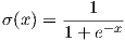
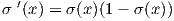
The advantage of structuring the activation function in this way is that it makes it easy to add other activation functions to the program as you can see in the full code. All that is required is that they are implemented as a class with two static methods; fn(x) which computes the activation function given input x, and prime(x) which computes the derivative of the activation function evaluated at x. An activation function class should assume that x is an instance of the Matrix class and ensure that operations are applied element-wise.

Feedforward


def feedforward(self, data):
        z = Matrix(data)
        for w, b in zip(self.weights[0:-1], self.biases[0:-1]):
            z = Matrix(self.activationfnHidden.fn(z * w + b))
        z = Matrix(self.activationfnLast.fn(z * 
                         self.weights[-1] + self.biases[-1]))
        return z.matrix

This function computes one pass of the data through the network. This setup supports batch inputs of any size. data is a 2D matrix, examples x features. The one idiosyncrasy of this implementation vs. others is that the computations for the last layer are outside the loop. This allows for a different activation function in the last layer should a user wish to implement this.

Loss (cost) function


class QuadraticCost:
    cost_type = "QuadraticCost"
    
    @staticmethod
    def compute_cost(output, y, lmda, weights):
        '''Cost function cost'''
        num_data_points = output.shape[0]
        diff = y - output
        
        '''Regularization cost'''
        sum_weights = 0
        for w in weights:
            sum_weights += 
                   np.sum(np.multiply(w.matrix,w.matrix))
        regularization = (lmda * sum_weights) 
                              / (num_data_points * 2)
        
        return  np.sum(np.multiply(diff, diff)) 
                      / (2 * num_data_points) + regularization
    
    @staticmethod
    def cost_prime(output, y):
        '''Derivative of the quadratic cost function'''
        return output - y

The first function compute_cost(output, y, lmda, weights) has two parts. The first part is the cost driven by the accuracy of the network when measured on the training data, i.e. the sum of the squared difference between output and y. The second part is a penalty for large weights. This particular implementation is known as L2 weight regularization and has the effect of shrinking the weights, making the output less sensitive to small perturbations in the input. In practice it helps to prevent the neural network from learning particularities of the training data and achieve better results on unseen data. For an explanation of why neural networks are regularized and an overview of different techniques available to network designers, see this post.

Let W be the set of weight matrices, and N be the number of datapoints. output and y are 2D matrices. Then putting these two parts together, the function that compute_cost(output, y, lmda, weights) implements is;

NNProgramInPython24x

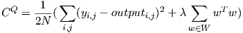
λ controls the extent of the regularization. λ = 0 corresponds to no regularization and λ = 1 corresponds to relatively strong regularization through a large additional penalty on the cost function.

cost_prime(output, y) computes the derivative of the cost function with respect to the output. The derivative of the regularization component of the cost function with respect to a weight matrix, w, is simply w. Since L2 regularization is used throughout this implementation regardless of the cost function, and to avoid cost prime returning a complicated list of partial derivatives, λw is subtracted from the current values of the weights when all of the parameters are updated in the update weights function.

Useful functions: Network predictions in a one hot encoded format and network accuracy for reporting


def predict(self, x):
        output = self.feedforward(x)
        if (output.shape[1]==1):
            '''If only one output, convert to 1 
               if value > 0.5'''
            low_indices = output <= 0.5             
            high_indices = output > 0.5
            output[low_indices] = 0
            output[high_indices] = 1
        else:
            '''Otherwise set maximum valued output 
               element to 1, the rest to 0'''    
            max_elem = output.max(axis=1)
            max_elem = 
              np.reshape(max_elem, (max_elem.shape[0], 1))
            output = np.floor(output/ max_elem)
        return output
    
def accuracy(self, x, y):
    prediction = self.predict(x)
    num_data_points = x.shape[0]
    if (prediction.shape[1]==1):
        result = np.sum(prediction==y) / num_data_points
    else:
        result = 
          np.sum(prediction.argmax(axis=1)==y.argmax(axis=1)) 
                                           / num_data_points
    return result

Predict converts the output nodes of a neural network to 1 if an example belongs to the class corresponding to that node, 0 otherwise. If there is only one output node then an output value >0.5 corresponds to that examples being a member of the positive class, otherwise it is a member of the negative class. If there are more than one output node then the node with the highest output value is converted to a 1 and the rest are set to 0.

Accuracy compares the network prediction to the correct results and returns the percentage of correctly classified examples.

Backpropagation


def backprop(self, x, y, lmda):
        num_data_points = x.shape[0]
        z_vals = []
        a_vals = [x]
        
        ''' Feedforward: storing all z and a values 
            per layer '''
        activation = Matrix(x)
        for w, b in zip(self.weights[0:-1], self.biases[0:-1]):
            z = activation * w + b
            z_vals.append(z.matrix)
            activation = Matrix(self.activationfnHidden.fn(z))
            a_vals.append(activation.matrix)
        z = activation * self.weights[-1] + self.biases[-1]
        z_vals.append(z.matrix)
        activation = Matrix(self.activationfnLast.fn(z))
        a_vals.append(activation.matrix)
              
        cost = self.costfn.compute_cost(a_vals[-1], y, 
                                      lmda, self.weights)
        cost_prime = self.costfn.cost_prime(a_vals[-1], y)
        
        ''' Backprop: Errors per neuron calculated first 
            starting at the last layer and working backwards 
            through the network, then partial derivatives 
            are calculated for each set of weights and biases
            deltas = neuron error per layer'''
        deltas = []
        
        if (self.costfn.cost_type=="QuadraticCost"):
            output_layer_delta = cost_prime * 
              self.activationfnLast.prime(Matrix(z_vals[-1]))
        elif (self.costfn.cost_type=="CrossEntropyCost"):
            output_layer_delta = cost_prime
        else:
            print("No such cost function")
            exit(1)
        
        deltas.insert(0, output_layer_delta)
        
        for i in range(1,self.layers-1):
            interim = np.dot(deltas[0], 
                     (np.transpose(self.weights[-i].matrix)))
            act_prime = 
             self.activationfnHidden.prime(Matrix(z_vals[-i-1]))
            delta = np.multiply(interim, act_prime)
            deltas.insert(0, delta)
        
        nabla_b = []
        for i in range(len(deltas)):
            interim = np.sum(deltas[i], axis=0) 
                                   / num_data_points
            nabla_b.append(np.reshape(interim, 
                                       (1, interim.shape[0])))
        
        nabla_w = []
        for i in range(0,self.layers-1):
            interim = np.dot(np.transpose(a_vals[i]), 
                                           deltas[i])
            interim = interim / num_data_points
            nabla_w.append(interim)
        
        return cost, nabla_b, nabla_w

The optimal parameter values in a neural network are found through the gradient descent. This is how a network learns. In each iteration of training, the neural network produces output via the feedforward function, computes the associated cost and calculates the partial derivatives of the cost function with respect to each of the parameter values. These values are then used to update the parameters, resulting in a small step in the direction of steepest gradient towards a lower cost. Backpropagation is the algorithm used to efficiently find the values of the partial derivatives and is an elegant application of dynamic programming and the chain rule of calculus.

Michael Nielsen’s explanation of backpropagation is superb, so I will not attempt to replicate it here. There are three steps to the algorithm:

  1. Calculate the error of each node, defined as the partial derivative of the cost with respect to the output of each node, before the activation function is applied
  2. Calculate the partial derivative of the cost with respect to the biases
  3. Calculate the partial derivative of the cost with respect to the weights

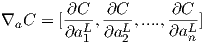
The terminology below is Michael Nielsen’s, see his chapter on backpropagation for more details (link above). Let’s define the error of the nodes in the output layer as δL, and the error of nodes in any other layer as δl. Define the output of nodes in a layer before the activation function is applied as zl, zL for the output layer. Finally, define the output of nodes in a layer after the activation function is applied as al, aL for the output layer. Finally, suppose there are n output nodes and define a C as the vector of the partial derivatives of the cost function with respect to aL, that is

NNProgramInPython25x

Let the derivative of the cost function be, σ'(x), ⊙ is the element wise multiplication operator, and wl is the weight matrix for layer l. Then the equation to calculate the error for each node is;

NNProgramInPython26x

NNProgramInPython27x

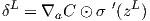
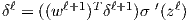
The errors are propagated backwards through the network from the output layer downwards. Errors are pushed down a layer by being multiplied with the relevant weights in the same layer and then the dot product is taken of the result and the derivative of the activation function in the layer below, evaluated at the input value to that function, zl. From here it is easy to calculate the relevant partial derivatives for the weights and biases.

NNProgramInPython28x

NNProgramInPython29x

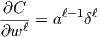
The first part of the backpropagation function calculates and stores all of the z and a values. Then δL (output layer delta) is calculated first, then the rest of the layers in a loop. Finally the partial derivatives with respect to the weights (nabla_w) and biases (nabla_b) are calculated and returned.

Parameter updates


def update_weights(self, nabla_w, nabla_b, 
                   learning_rate, lmda, num_data_points):
        i = 0
        weight_mult = 1 - ((learning_rate * lmda) 
                                   / num_data_points)
        for w, nw in zip(self.weights, nabla_w):
            self.weights[i].matrix = weight_mult * w.matrix 
                                          - learning_rate * nw
            i += 1
        i = 0
        for b, nb in zip(self.biases, nabla_b):
            self.biases[i].matrix = b.matrix 
                                          - learning_rate * nb
            i += 1

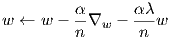
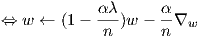
This is a fairly self explanatory function. It controls the updates to the weights and biases. The biases update is straightforward, depending only on the values of the current weights, learning rate and gradients (nabla_b). The weight updates are a little more complex since they also includes the regularization component. Let λ be the variable lmda, α be the learning rate, and n be the number of data points. Then the function it computes is

NNProgramInPython210x

NNProgramInPython211x

Note: nabla_w and nabla_b have already been divided by the number of data points in the backpropagation function so there is no need to do so in this function.

Stochastic Gradient Descent


def SGD(self, x, y, valid_x, valid_y, learning_rate, epochs, 
        reporting_rate, lmda=0, batch_size=10, verbose=False):
        training_cost = []
        valid_cost = []
        num_data_points = batch_size
        total_data_points = x.shape[0]
        output = self.feedforward(x)
        cost = self.costfn.compute_cost(output, y, 
                                     lmda, self.weights)
        accuracy = self.accuracy(x, y)
        valid_accuracy = self.accuracy(valid_x, valid_y)
        print("Training cost at start of training is %.5f 
               and accuracy is %3.2f%%" % (cost, accuracy * 100))
        print("Validation set accuracy is %3.2f%%" % 
                                  (valid_accuracy * 100))
        if (verbose==True):
            print("First 10 output values are:")
            print(output[0:10,:])
        
        for i in range(epochs):
            data = np.hstack((x,y))
            input_dims = x.shape[1]
            output_dims = y.shape[1]
            np.random.shuffle(data)
            batches = []
            nabla_w =[]
            nabla_b = []
            
            for k in range(0, (total_data_points - batch_size), 
                                                    batch_size):
                batch = data[k:(k+batch_size),:]
                batches.append(batch)
            num_batches = len(batches)
            for j in range(num_batches):
                batch_x = batches[j][:,:input_dims]
                batch_y = batches[j][:,input_dims:]
                if (batch_y.ndim == 1):
                    batch_y = np.reshape(batch_y, 
                                          (batch_y.shape[0],1))
                cost, nabla_b, nabla_w = 
                             self.backprop(batch_x, batch_y, lmda)
                self.update_weights(nabla_w, nabla_b, 
                             learning_rate, lmda, num_data_points)

                '''Monitoring progress (or lack of...)'''
                training_cost.append(cost)
                valid_output = self.feedforward(valid_x)
                valid_c = self.costfn.compute_cost(valid_output, 
                                        valid_y, lmda, self.weights)
                valid_cost.append(valid_c)
            
            if (i % reporting_rate == 0):
                output = self.feedforward(x)
                cost = self.costfn.compute_cost(output, 
                                             y, lmda, self.weights)
                accuracy = self.accuracy(x, y)
                valid_accuracy = self.accuracy(valid_x, valid_y)
                print("Training cost in epoch %d is %.5f and 
                       accuracy is %3.2f%%" % (i, cost, 
                       accuracy * 100))
                print("Validation set accuracy is %3.2f%%" % 
                                         (valid_accuracy * 100))
                if (verbose==True):
                    print("First 10 output values are:")
                    print(output[0:10,:])
                    print("Weight updates")
                    for i in range(len(self.weights)):
                        print(nabla_w[i])
                    print("Bias updates")
                    for i in range(len(self.biases)):
                        print(nabla_b[i])
                    print("Weights")
                    for i in range(len(self.weights)):
                        print(self.weights[i].matrix)
                    print("Biases")
                    for i in range(len(self.biases)):
                        print(self.biases[i].matrix)
                
        '''Final results'''
        output = self.feedforward(x)
        cost = self.costfn.compute_cost(output,y,lmda,self.weights)
        prediction = self.predict(x)
        accuracy = self.accuracy(x, y)
        valid_accuracy = self.accuracy(valid_x, valid_y)
        print("Final test cost is %.5f" % cost)
        print("Accuracy on training data is %3.2f%%, and 
              accuracy on validation data is %3.2f%%" %
              (accuracy * 100, valid_accuracy * 100))  
        
        return training_cost, valid_cost

Stochastic gradient descent puts everything together. After initializing the class and calling one of the variable initializer functions, all you need to do to train the neural network is to call SGD. When SGD returns, the values of the weights and biases will have been updated to the (hopefully) good values that the network found through stochastic gradient descent. Its main role is to create the batches based on the batch size, shuffling the data at the beginning of each epoch, call the backprop and update_weights function on each batch, and report on progress. The verbose parameter controls whether some of the internals of the network are printed out during training. This was mainly useful for debugging the program as I built it and is intended for network of toy sizes (only a few nodes per layer and a few data examples). It helped me to check that the prediction and accuracy functions were correct, that regularization was working as expected, and to pinpoint errors caused by underflow and overflow. It was also interesting to monitor the values of the outputs and weights as very small networks learned.

The SGD function sets all of the hyperparameters:

  • x: training data
  • y: training labels
  • valid_x: validation data
  • valid_y: validation labels
  • learning_rate: hyperparameter controlling the size of the parameter updates
  • epochs: number of complete iterations through the training data
  • reporting_rate: how frequently to report the training data cost and accuracy, and validation data accuracy. If epoch % reporting_rate == 0 the results are printed
  • lmda: regularization parameter. lmda = 0 corresponds to no regularization
  • batch_size: size of the batches used in one feedforward and parameter update step
  • verbose: True or False. True prints internal model statistics to the screen.

This code is all you need for a reasonably powerful feedforward neural network. The full program is available here. Not all combinations of cost functions and activation functions in the output layer will work. Different options should be paired as follows:

  • Sigmoid + Quadratic
  • Sigmoid + Cross Entropy (tends to learn much faster than Sigmoid + Quadratic)
  • Softmax + Log Likelihood

ReLU and LeakyReLU should only be used in the hidden layers, and Softmax is best used only in the output layer. Different network architectures, training data size, activation and cost functions, and batch sizes all require different learning rates and regularization strength to achieve good performance. See my next post, A Neural Network Program in Python: Part 2 for some examples.

I hope that you’ve enjoyed this post and found it useful. If you have any feedback please send me an email at contact@learningmachinelearning.org

Regularization for Neural Networks

Regularization is an umbrella term given to any technique that helps to prevent a neural network from overfitting the training data. This post, available as a PDF below, follows on from my Introduction to Neural Networks and explains what overfitting is, why neural networks are regularized and gives a brief overview of the main techniques available to a network designer. Weight regularization, early stopping, and dropout are discussed in more detail.

Regularization for Neural Networks PDF

Introduction to Neural Networks

   Neural networks burst into the computer science common consciousness in 2012 when the University of Toronto won the ImageNet[1] Large Scale Visual Recognition Challenge with a convolutional neural network[2], smashing all existing benchmarks. In the same year, Andrew Ng worked with Google to build the largest neural network to date. Trained on 10 million YouTube videos, the network learnt to recognize objects, cats most famously, without ever being given labelled examples. Better and better results quickly followed and computer vision was changed forever. More recently, neural networks have achieved state of the art results in natural language processing, have composed music[3], beat the human world champion at Go[4], and now power Google’s search algorithm[5].

In their modern form, neural networks have existed since the 1980’s. 1989 saw a breakthrough result when Yann LeCun successfully trained a neural network to recognize handwritten zip codes. Constrained by a lack of data and computing power, neural networks were superseded by other machine learning algorithms in the 1990s and most researchers moved on. Their startling resurgence and rapid domination of the machine learning field is enough for neural networks to be of interest to any data scientist and machine learning researcher. However it is their elegance, flexibility and generality that make them so fascinating to study. By giving up some control over what and how algorithms learn, computer science has gained the most powerful predictive algorithm in history.

This post is an introduction to neural networks for a reader with no background in neural networks or machine learning. It is the first in a series of four articles on neural networks. It does assume a basic understanding of linear algebra and calculus. If you are comfortable with vectors, matrices, the dot product, matrix-vector multiplication, matrix-matrix multiplication, transposing vectors and matrices, element wise operations, norms, partial derivatives and second order partial derivatives then you will be fine. By the end of it a reader should have a good understanding of what the fundamental components of a neural network are, how they are combined, how a neural network makes a prediction, and how it learns to produce good results. This post focuses on helping a reader develop good intuition for why different choices have been made in the design of neural networks, and  contains an in depth discussion of the role of the activation function. It is organized into four sections and is available as a PDF (link below)

  1. What is a neural network?
  2. Historical motivations for neural networks
  3. Role of the activation function
  4. How a neural network learns

Introduction To Neural Networks PDF

Later articles in this series will discuss regularization and provide a practical example of how to build your own neural network program in Python. Here is a quick preview of what is to come:

  • Regularization for Neural Networks: Explanation of regularization and an overview of the main techniques.
  • A Neural Network program in Python: Walk through of a vectorized implementation of a general neural network program with examples. With it you will be able to build an arbitrary sized network and choose from different cost, activation, and parameter initialization functions.

[1] ImageNet challenge website

[2] See this technology review article and ImageNet Large Sale Visual Recognition Challenge, Russakovsky et. al., 2015 for more details

[3] Jukedeck

[4] AlphaGo

[5] For more information on the history of machine learning and neural networks, watch Frank Chen’s video

Principal Component Analysis

Principal Component Analysis (PCA) is a popular dimensionality reduction technique and the maths behind it is very elegant. However, it was difficult to find worked examples that clearly demonstrated when using PCA is helpful during data analysis. It is often used to visualize datasets by projecting features onto 2 or 3 dimensional space. However, I also wanted to understand if using PCA before fitting a linear model could lead to better results. I conducted experiments with toy datasets and a small real dataset to address this question. This post contains the results. It is intended to explain what PCA is and to explore when it is and is not useful for data analysis.

Section one explains the mathematics of PCA. PCA is the process of transforming a dataset, X, into a new dataset Y. The section starts with the desirable properties of the transformed dataset, Y, and works through the mathematics which guarantee these properties. It is intended to be understood by a reader who has a basic understanding of linear algebra, but can be skipped if readers wish only to see the application of PCA to datasets.

Section two uses toy datasets to demonstrate what happens to the principal components and the accuracy of a simple principal component regression when the variance of features change.

Section three explores the trade off between dimensionality reduction using PCA and the performance of a linear model. It compares the performance of linear regression, ridge regression and principal component regression in predicting the median household income of US counties. The objective of this section is to show how the accuracy of principal component regression changes as the number of principal components is reduced, and to assess how effective PCA is in preventing overfitting when compared to ridge regression.

The full post (pdf), appendix (pdf), and link to the MATLAB code is below. If you have any feedback please email: contact [at] learningmachinelearning [dot] org

PCA_LG_Mar16

PCA_LG_Appendix_Mar16

Matlab Code